Vector Quantization: The Mathematical Art of Audio Compression

Every sound is data of millions of samples every second. Compressing all that without losing clarity has always been the challenge. Now imagine if a model could learn what truly matters in those waves and ignore the rest. That idea, called vector quantization, reshaped how modern AI handles voice and music.

The Challenge Behind Modern Audio Compression

Modern voice AI systems face a big challenge: every second of CD-quality audio produces about 1.4 million data points. Multiply that by millions of users, and storage and transmission quickly become expensive. Earlier compression techniques such as MP3, AAC, and Opus helped, but each involved trade offs reducing bandwidth at the cost of quality or latency.

A simpler idea was treating sounds as a continuous stream of data points. But what if we could represent these sounds more efficiently?

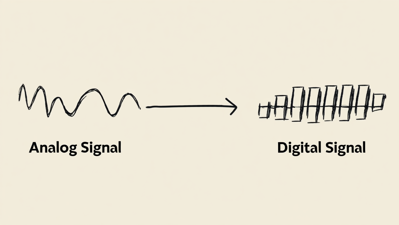
Figure 1: Continuous vs. Discrete Signal Representation

Understanding Quantization

Before we jump into how audio uses quantization, it helps to understand what quantization means in machine learning. In Machine learning, quantization refers to reducing the precision of numbers used to represent model parameters or activations like converting 32-bit floating points to 8-bit integers.

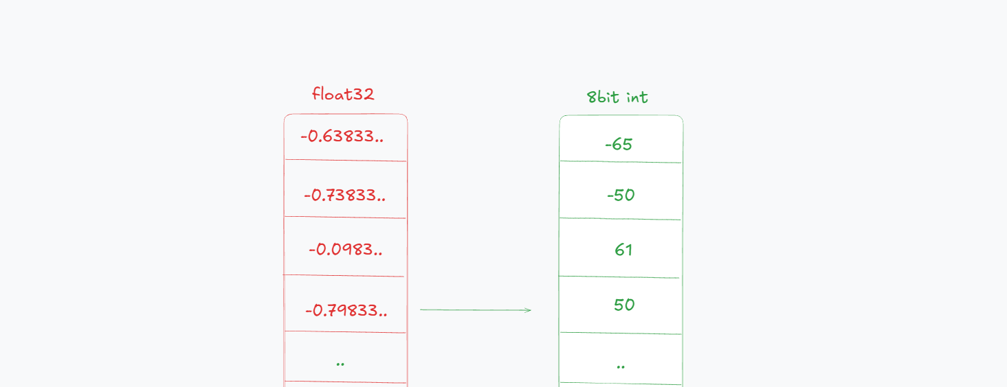
Figure 2: 32-bit Float to 8-bit Integer Quantization

NOTE: Quantization is different from compression. Compression reduces the size of data by encoding it more efficiently, while quantization reduces the precision of data representation.

This makes models faster and lighter, but it is a win win game if we are constrained on a limited amount of compute by sacrificing a small amount of accuracy for big efficiency gains. While this approach works well for neural networks, audio data has unique properties that require a more sophisticated strategy—one that can capture the complex patterns hidden in sound waves.

Vector Quantization Through Speech

Enter vector quantization, a technique that transforms high-dimensional audio data into compact representations without significant loss of quality. Vector quantization (VQ) exploits the fact that variation in natural data is redundant. When you hear someone say "hello", your brain doesn't process every microscopic detail of the sound wave. Instead, it extracts key features and matches them against learned patterns.

Let's break down how VQ works mathematically.

Given input vector x ∈ ℝⁿ, find codebook entry cᵢ that minimizes:

$d(x, c_i) = ||x - c_i||^2$

Let's say we have a 256-dimensional vector representing a short audio segment. Instead of storing all 256 values, we can use VQ to find the closest match from a learned codebook of common speech patterns.

import numpy as np

# Audio segment encoded as 256-dimensional vector
audio_vector = np.array([0.23, -0.41, 0.67, -0.12, ...])  # 256 values

# Learned codebook representing common speech patterns
codebook = np.array([
    [0.25, -0.40, 0.65, -0.10, ...],  # maybe a fricative sound
    [0.15, 0.32, -0.21, 0.45, ...],   # maybe a vowel sound
    [0.67, -0.23, 0.12, 0.89, ...],   # maybe a plosive sound
])

def quantize_vector(input_vec, codebook):
    """Find closest codebook match using L2 distance"""
    distances = np.linalg.norm(codebook - input_vec, axis=1)
    best_index = np.argmin(distances)
    return codebook[best_index], best_index

quantized_vec, index = quantize_vector(audio_vector, codebook)
# Store index (small integer) instead of 256 floats

By storing just the index of the closest codebook entry, we drastically reduce the amount of data needed to represent the audio segment.

How the Codebook is Learned

Traditional approaches used k-means clustering to discover representative patterns:

def learn_codebook_kmeans(training_data, k=1024):
    # Initialize random centroids
    centroids = np.random.randn(k, vector_dim)

    for iteration in range(max_iters):
        # Assign each vector to nearest centroid
        assignments = []
        for vec in training_data:
            distances = np.linalg.norm(centroids - vec, axis=1)
            assignments.append(np.argmin(distances))

        # Update centroids as cluster means
        for i in range(k):
            cluster_vecs = training_data[np.array(assignments) == i]
            if len(cluster_vecs) > 0:
                centroids[i] = np.mean(cluster_vecs, axis=0)

    return centroids

Newer codecs use more sophisticated methods like VQ-VAE to jointly learn the codebook and the encoder-decoder architecture.

This worked for offline processing but had serious limitations for neural network training. The discrete assignment steps and batch processing requirements made gradient-based optimization difficult.

Limitations of Traditional Vector Quantization

Let the input be a feature vector $\mathbf{x} \in \mathbb{R}^d$ and a finite codebook $\mathcal{C} = \lbrace \mathbf{c}_1, \mathbf{c}_2, \dots, \mathbf{c}_K \rbrace$. Vector quantization replaces each input with its nearest codeword:

$Q(\mathbf{x}) = \arg\min_{\mathbf{c}_k \in \mathcal{C}} \|\mathbf{x} - \mathbf{c}_k\|_2^2$

The expected distortion (error) is:

$D = \mathbb{E}_{\mathbf{x}}\left[\|\mathbf{x} - Q(\mathbf{x})\|_2^2\right]$

Core Limitations

1. Limited expressiveness — A single codeword per region can't capture complex or multimodal distributions in $p(\mathbf{x})$.
2. Codebook growth problem — To halve distortion, you often need to square the number of codewords: $D \propto K^{-2/d}$. Larger $K$ implies exponential memory and compute.
3. High encoding cost — Nearest-neighbor search costs $O(Kd)$ for each vector.
4. No residual correction — Once quantized, the residual $\mathbf{e} = \mathbf{x} - Q(\mathbf{x})$ is discarded, wasting useful fine-grained detail.
5. Uniform distortion metric — Standard L2 distance treats all dimensions equally.

Classic VQ minimizes distortion but scales poorly with dimension and distribution complexity — this motivates techniques like Residual Vector Quantization (RVQ) to address these limitations.

Residual Vector Quantization

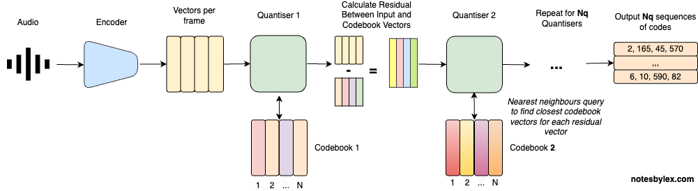
Figure 3: Residual Vector Quantization (RVQ) Architecture

Residual Vector Quantization fundamentally changed the game by stacking multiple quantizers, where each stage learns to encode the error left behind by the previous one.

The mathematical formulation of RVQ is:

$\mathbf{x} \approx q_1(\mathbf{x}) + q_2(\mathbf{x} - q_1(\mathbf{x})) + q_3(\mathbf{x} - q_1(\mathbf{x}) - q_2(\mathbf{x})) + \ldots$

where:

• $\mathbf{x} \in \mathbb{R}^d$ is the input vector
• $q_i(\cdot)$ is the quantizer at stage $i$
• $\mathbf{r}_i = \mathbf{x} - \sum_{j=1}^i q_j(\mathbf{r}_{j-1})$ is the residual at stage $i$

The final reconstruction is:

$\hat{\mathbf{x}} = \sum_{i=1}^N q_i(\mathbf{r}_{i-1})$

RVQ builds the final approximation by adding up several small corrections instead of using one big codebook.

def residual_quantize(input_vec, codebooks):
    """Multi-stage quantization with progressive refinement"""
    reconstruction = np.zeros_like(input_vec)
    residual = input_vec.copy()
    indices = []

    for stage, codebook in enumerate(codebooks):
        quant_vec, idx = quantize_vector(residual, codebook)
        reconstruction += quant_vec
        indices.append(idx)
        residual = input_vec - reconstruction
        print(f"Stage {stage+1} residual norm: {np.linalg.norm(residual):.4f}")

    return reconstruction, indices

Audio Demonstrations

Original Audio

4 Codebooks Reconstruction

8 Codebooks Reconstruction

16 Codebooks Reconstruction

32 Codebooks Reconstruction

Bitrate Control Through RVQ

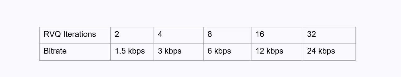
Figure 4: RVQ in EnCodec — Bitrate Control Through Multiple Quantization Stages

One of the biggest advantages of RVQ is fine-grained control over bitrate. By adjusting the number of quantization stages or the size of each codebook, we can trade off quality versus compression.

Meta's EnCodec paper demonstrated the practical power of this approach.

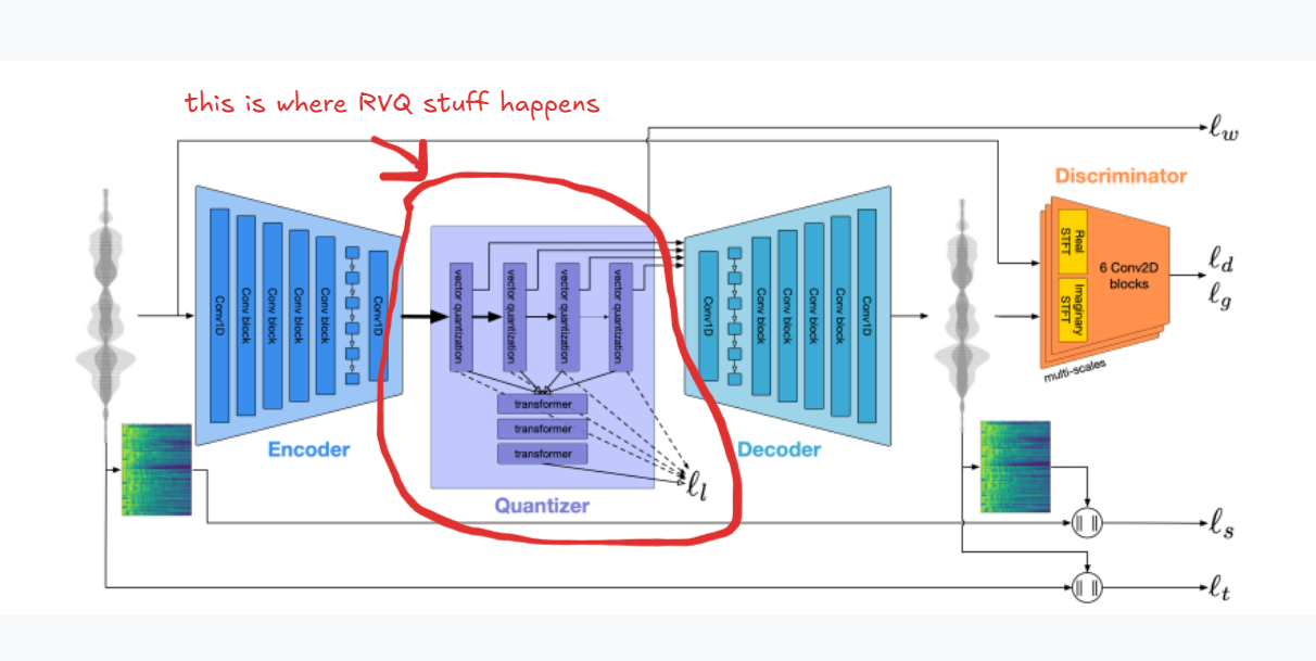
Figure 5: Meta's EnCodec Architecture

The mathematical relationship shows exponential growth in representational capacity:

$\text{Total patterns} = 2^{b \times N}$

where $b$ is bits per stage and $N$ is the number of stages.

Exponential Moving Average (EMA) Codebook Update

To stabilize training, each codeword is updated using an exponential moving average:

$\mathbf{c}_i^{(t+1)} = \alpha \, \mathbf{c}_i^{(t)} + (1 - \alpha) \, \bar{\mathbf{v}}_i$

where:

• $\mathbf{c}_i^{(t)}$ is the codeword at iteration $t$
• $\bar{\mathbf{v}}_i$ is the mean of all encoder outputs assigned to codeword $i$
• $\alpha \in [0, 1)$ is the momentum parameter (typically 0.99)

A higher $\alpha$ means slower, smoother updates; lower values adapt faster but can be noisy. This EMA rule helps the codebook evolve continuously, reducing abrupt jumps and preventing codeword collapse.

References

1. Défossez, A., Copet, J., Synnaeve, G., & Adi, Y. (2022). High Fidelity Neural Audio Compression. arXiv:2210.13438
2. Zeghidour, N., et al. (2021). SoundStream: An End-to-End Neural Audio Codec. Google Research
3. AssemblyAI. What is Residual Vector Quantization? assemblyai.com
4. Notes by Lex. Residual Vector Quantisation. notesbylex.com
5. Yannic Kilcher. High Fidelity Neural Audio Compression (EnCodec Explained). YouTube